
Introduction
In response to my approach in the popular MDX Guide for SQL Folks series, I am using SQL as a good frame of reference for starting or developing a new approach for improving your Data Analysis Expression(DAX) language learning experience. This is useful for developers starting to learn the DAX language to more advanced developers who have struggled to adjust to the language coming from a SQL background.
In Part I of the series, we discussed some very important Data Visualization and Tabular Model concepts that are essential to the DAX learning process, esp. when coming from a SQL background;
- First, we discussed the importance of learning and applying Data Visualization techniques. We learned that applying these can increase one's potential to effectively communicate decision making insights to drive action. There are many books available that teach this art and science of analytical storytelling.
- We also learned the benefits of interactive visualization that comes with tools like Power BI. Interactive visualization tools take the concept of data visualization a step further by using data modeling and technology to enable end-user to drill down into visuals to fully explore and analyze data.
- We examined the key similarities and differences between and a SQL Server Database and the Tabular Model that power T-SQL and DAX respectively. We learned that:
- In both databases the basic elements are tables, but in a SQL Server Database, tables are isolated units whilst in Tabular Models, tables are all joined into one physical data model.
- Because tables are left joined to other tables on the many-to-one side, tables in Tabular Models are essentially Extended Tables.
- Understanding the Extended Tables and other Tabular Models concept is key. It will help one to grasp the effects of DAX relationships, filter propagation, interactivity and their effects on the DAX formulas and expression that you will write.
- Finally, we learned that, even though both DAX and SQL languages can achieve the same query results, SQL is a Declarative Language whilst DAX is a Purely Functional Language. Knowing and always keeping this last point in mind and also understanding how functional language syntax is constructed makes transitioning from SQL to DAX a lot easier.
If you have not done so yet, please refer to Part I, especially for the concept outlined in bullet points 3 and 4, they form the foundation of this learning process.
In Part II we are going to continuing to learn DAX by solidifying our understanding of its functional nature compared to the declarative nature of SQL. We will learn how the pre-built relationship between tables in a Tabular Model affects DAX language as opposed to using join statements in SQL simply because tables in SQL Server databases are not joined to each other. We will do this by simply translating SQL queries to DAX queries.
Part II: SQL Queries vs DAX Queries
We are going to make the initial learning process simple and straight forward by comparing SQL and DAX queries. We will introduce SQL clauses and syntax first followed by their DAX equivalent. We will look at how the SQL clauses in the Logical SQL query processing steps below translated into DAX as a functional language.
Logical SQL query processing steps
(4) SELECT (4-2) DISTINCT (4-3) TOP(<top_specification>) (4-1) <select_list>
(1) FROM <left_table> <join_type> JOIN <right_table> ON <on_predicate>
(2) WHERE <where_predicate>
(3) GROUP BY <group_by_specification>
(5) ORDER BY <order_by_list>;
By following and understanding the translation of the Logical SQL query processing steps above into functional DAX syntaxes, you would have learned a lot about what you need to know about DAX. Most resources on this topic do not teach or emphasize the functional nature and syntax of DAX so learners leave without a very key element. We are going to emphasize this in this section with Summarized Functional Syntaxes that ignores non-functional arguments.
As we translate SQL to DAX functional syntax, one should understand that logically the inner functions are processed first and passed on to the next ones in the function chain, as opposed to the numbered SQL query processing steps shown above.
Database Installation
For those who want to follow the examples by executing both the SQL and DAX queries you can do that by installing the AdventureWorksDW SQL Server and SSAS Tabular Model sample databases.
- To download and install the Data Warehouse versions of the AdventureWorks SQL Server sample database you can follow the example in this link.
- To download and install the AdventureWorks Tabular Model sample database you can follow the examples in the links below.
SQL and DAX Client Query Tools
Most readers on this forum should be familiar with SSMS. SSMS is the primary client tool for querying SQL Server Databases. After installing the AdventureWorks Tabular Model sample database , one can also connect to the database and run DAX queries using SSMS by following the steps in figure 1 below.
- First, click on the DAX query button in SSMS.
- This will launch the screen that lets you select and connect to the SSAS Server with the Tabular Database you install above.
- Make sure you select the database you want to query
- Proceed to write and execute your DAX queries
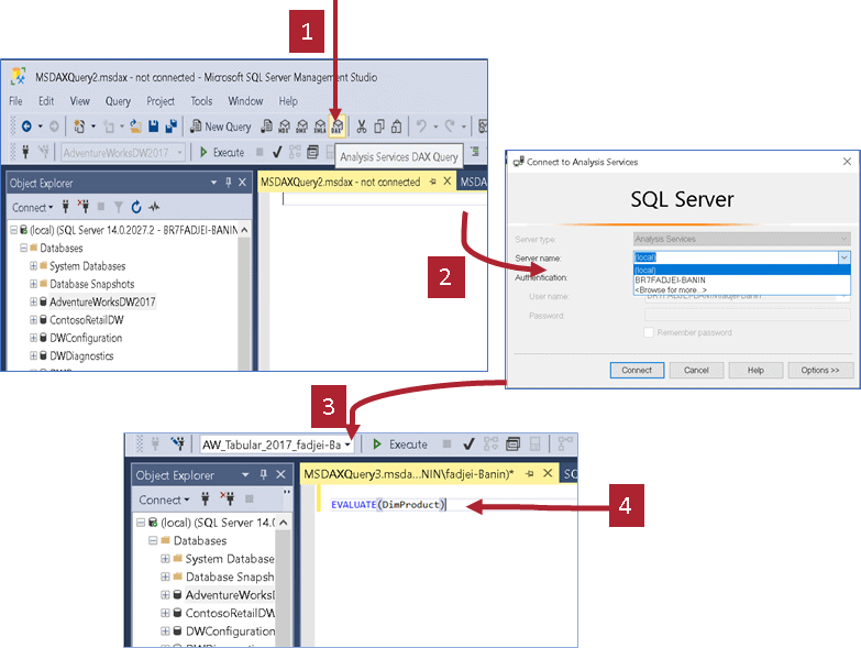
figure 1: Showing how to connect to SSAS Tabular Databases and write DAX queries.
However, if you are going to run a lot of ad-hoc DAX queries and test DAX calculations and expressions, then I suggest you install and use DAX Studio since it offers more DAX features, like formating. Please visit http://daxstudio.org to read the full documentation and download the latest release of DAX Studio.
DAX Table and Column Name Syntax
It is important to know the general format for referencing table and columns in DAX, as shown below;
            'Table Name'                   //  Table  reference
            'Table Name'[Column Name]      //  Column reference
If the table name has no spaces, the single quotes can be omitted, so the syntax looks like below:
TableName[Column Name]
In this series, we are going to use the quoted version whether the table name has spaces or not.
DAX Functions Reference
We will encounter new DAX functions as we go along. For these discussions, a few key ones will be partially introduced. For an in-depth look at any function, one can follow the links provided below.
These function references provide detailed information including syntax, parameters, return values, and examples for each of the functions that will be used DAX queries and formulas in this series.
SQL SELECT FROM Clauses vs DAX EVALUATE Function
Just like you need the SELECT FROM statement in SQL to query tables in a Relational Database, in DAX if you need the EVALUATE function to query the data in a tabular model. Let's start with a simple statement by querying the DimProduct Table in both databases with SQL and DAX.
Listing 1:
SQL:
Select * From DimProduct
DAX:
EVALUATE('DimProduct')
Both queries in Listing 1 above return all the rows from the DimProduct table. From the DAX query, we see the use of the EVALUATE function, which is the only required function for querying in DAX. Note that EVALUATE was not used with any column projection function so the effect is similar to SELECT * FROM.
Intro to the EVALUATE Function
To query data directly in a tabular model, you need the EVALUATE function. The EVALUATE function is used to return the result set as a table. It is the equivalent to using SELECT FROM statement in T-SQL to return columns and rows from a table.
EVALUATE('table name')
In this expression 'table name' refers to the name of a table, a table function, or an expression that returns a result set.
Note: Every time you have a DAX function that accepts a table expression as an argument, you can write the name of a table in that parameter, or you can write a function or an expression, that returns a table.
Let's explore the functional nature of DAX a bit further. In the next logic, we will query the top 5 records from the DimProduct table as shown in Listing 2 below.
Listing 2:
SQL:
SELECT TOP(5)
        *
FROM DimProduct
DAX:
EVALUATE(TOPN(5,'DimProduct'))
TOPN is DAX equivalent of the SQL TOP function, as you can see from Listing 2, the TOPN function is just nested within the EVALUATE function as below, illustrating the functional syntax of DAX.
Summarized Functional Syntax:
EVALUATE(TOPN())
SQL WHERE Clause vs the DAX FILTER Function
The DAX FILTER Function is the function used to achieve the effects of the WHERE clause in the SQL query logical steps.
In the following example, we will write a query to restrict the top 5 records from the DimProduct table to where the color of the product is black and the status of the product is marked as current. The SQL and DAX equivalent of this logic is as shown in Listing 3 below.
Listing 3:
SQL:
SELECT TOP(5)
        *
FROM   DimProduct
WHERE  [DimProduct].[Color]='Black'
AND    [DimProduct].[Status] ='Current'
DAX (unformatted):
EVALUATE(TOPN( 5, ( FILTER( 'DimProduct', 'DimProduct'[Color] = "Black" && 'DimProduct'[Status] = "Current" ) ) ) )
DAX(formatted):
EVALUATE
 (
    TOPN (
        5,
        (
            FILTER (
                'DimProduct',
                'DimProduct'[Color] = "Black"
                    && 'DimProduct'[Status] = "Current"
            )
        )
    )
)
Two options of the DAX query are shown in Listing 3: an unformatted single line and a more functional, formatted version. The versions are to illustrate the point that, no matter how complex it is, a DAX expression is like a single function call as shown in the functional syntax below.
Summarized Functional Syntax:
EVALUATE(TOPN((FILTER())))
The complexity of the DAX code comes from the complexity of the expressions that one uses as parameters for the outermost function.
DAX Formatting
As formulas start to grow in length and complexity, it is extremely important to format the code to make it human-readable. Functional language formatting follow certain rules and could be a time-consuming operation. The Folks at SQLBI created a free tool can that transform your raw DAX formulas into clean, beautiful and readable formatted code. You can find the website at www.daxformatter.com. On the website, you can also learn the syntax rules used to improves the readability DAX expressions.
Intro: FILTER Function
The filter function is one of the most important DAX functions you will encounter. The FILTER function, however, has a very simple role: it is an iterator table function. It gets a table, iterates over the table and returns a table that has the same columns as in the original table, but contains only the rows that satisfy a filter condition applied row by row.
The syntax of FILTER is the following;
FILTER (<table>, <condition>)
FILTER iterates the <table> and, for each row, evaluates the <condition>, which is a Boolean expression.When the <condition> evaluates to TRUE, the FILTER returns the row; otherwise, it skips it.
Note From a logical point of view, FILTER executes the <condition> for each of the rows in <table>. However, internal optimizations in DAX might reduce the number of these evaluations up to the number of unique values of column references included in the <condition> expression. The actual number of evaluations of the <condition> corresponds to the “granularity” of the FILTER operation. Such a granularity determines FILTER performance, and it is an important element of DAX optimizations.
SQL ORDER BY Clause vs DAX ORDER BY Parameter
The DAX Order By keywords or optional parameter is similar to the SQL Order By keywords. The query in Listing 4 below shows how the previous result set from the DimProduct table is ordered by EnglishProductName.
Listing 4:
SQL:
SELECT TOP(5)
          *
FROM     [DimProduct]
WHERE    [DimProduct].[Color]='Black'
AND      [DimProduct].[Status] ='Current'
ORDER BY [DimProduct].[EnglishProductName]
DAX:
EVALUATE
 (
    TOPN (
        5,
        (
            FILTER (
                'DimProduct',
                'DimProduct'[Color] = "Black"
                    && 'DimProduct'[Status] = "Current"
            )
        )
    )
)
ORDER BY 'DimProduct'[EnglishProductName]
Note that in DAX ORDER BY is not a function; it is rather an optional parameter of EVALUATE function.
Summarized Functional Syntax:
EVALUATE(TOPN((FILTER())))
ORDER BY
SQL Select_list vs DAX Projection Functions
In SQL, the select_list enables you to outline the columns you want in your query result set, as in;
SELECT column1, column2,…. FROM
In DAX there are a couple of functions you could use to project table columns to achieve the same results as SQL select_list. For DAX querying purposes we will use the very efficient SUMMARIZECOLUMNS function which has been designed to be the “one function fits all” to run queries.
The example that follows shows a simple query to illustrate the use of SUMMARIZECOLUMNS function. The queries show how to project EnglishProductName and Color columns from the DimProduct table.
Listing 5:
SQL:
SELECT
         [EnglishProductName] ,
         [Color]
FROM DimProduct
DAX (Option 1):
EVALUATE
 (
    SUMMARIZECOLUMNS (
        'DimProduct'[EnglishProductName],      // column name
        'DimProduct'[Color],                   // column name

        'DimProduct'                           // Base Table name
    )
)
DAX (Option 2) :
EVALUATE
 (
    SUMMARIZECOLUMNS (
        'DimProduct'[EnglishProductName],  // column name
        'DimProduct'[Color]                // column name
    )
)
As we can see from the listing above there are two options of the query for DAX, Option 1 with the name of the table and Option 2 without the name of the table.
Note that option 2 works and it goes to show that the table expression is optional. However, when selecting from multiple tables you must specify the base table to use for the join operation, if not you obtain a cross join. On the other hand, if there is an aggregation expression in your query, the DAX engine would infer the base table from the aggregation expression. In this series, we are going to use the first option by always specifying the base table whether projecting from one or more tables.
Let's try a more complex logic by selecting columns in our previous queries from Listing 4 as shown in Listing 6 below.
Listing 6:
SQL:
SELECT TOP(5)
         [EnglishProductName] ,
         [Color]
FROM     DimProduct
WHERE    DimProduct.[Color]='Black'
AND      DimProduct.[Status] ='Current'
ORDER BY DimProduct.[EnglishProductName]
DAX:
EVALUATE
 (
    TOPN (
        5,
        (
            SUMMARIZECOLUMNS (
                'DimProduct'[EnglishProductName],
                'DimProduct'[Color],
                FILTER (
                    'DimProduct',
                    'DimProduct'[Color] = "Black"
                        && 'DimProduct'[Status] = "Current"
                )
            )
        )
    )
)
ORDER BY 'DimProduct'[EnglishProductName]
Summarized Functional Syntax:
EVALUATE(TOPN(SUMMARIZECOLUMNS(FILTER())))
ORDER BY
SQL GROUP BY Vs DAX Aggregation
Unlike SQL, where you have to explicitly state the group by clause, in DAX the feature is built into SUMMARIZECOLUMNS and other column projection functions. The group by feature is forced by the introduction of an aggregation function within the SUMMARIZECOLUMNS function as shown in Listing 7 below.
Listing 7:
SQL:
SELECT salesordernumber,
       Sum([salesamount])AS 'SumOfSales'
FROM   FactResellersales
GROUP  BY salesordernumber
DAX:
EVALUATE
 (
    SUMMARIZECOLUMNS (
        'FactResellerSales'[SalesOrderNumber],
        'FactResellerSales',
        "SumOfSales", SUM ( 'FactResellerSales'[SalesAmount] )
    )
)
Summarized Functional Syntax:
EVALUATE( SUMMARIZECOLUMNS( SUM() ) )
As we can see from the DAX logic in Listing 7 above, by the mere introduction of the SUM function, SUMMARIZECOLUMNS function knows to group by the projected columns. Always remember that you must specify table expression argument after the columns you projecting and before the aggregated or calculated columns.
Intro: SUMMARIZECOLUMNS Function
We've learned that SUMMARIZECOLUMNS is an extremely powerful query function with all the features needed to execute a query. It returns a summary table over a set of groups. SUMMARIZECOLUMNS lets you specify:
- A set of new columns to add to the result.
- A set of columns used to perform Group-By, with the option of producing subtotals. SUMMARIZECOLUMNS automatically groups data by selected columns. The result is equivalent to SQL Select Distinct.
- A set of filters to apply to the model before performing the group-by.
- You must specify the table expression argument after the columns you projecting and before the aggregated or calculated columns.
- SUMMARIZECOLUMNS automatically removes from the output any row for which all the added columns produce a blank value.
- In SUMMARIZECOLUMNS you can add multiple filter tables, which could be useful for queries applied to complex data models with multiple fact tables.
- Because of this aggregating feature SUMMARIZECOLUMNS always return a distinct number of record
SQL Joins vs DAX Relationships
In Part I, we learned that in SQL Server databases, tables are isolated units whilst in Tabular Models, tables are all joined into one physical data model. When you build a tabular model, the relationships you define between tables at design time get established as actual relationships because the DAX engine joins all the tables together with a left join. So essentially, tabular model tables are extended tables. Please refer to Part I of the series where these concepts are well explained.
What these concepts mean is that unlike SQL where you specify joins within the query, DAX uses an automatic LEFT OUTER JOIN in the query whenever you use columns related to the primary table (the table on the left side of the Join.
Let's see how these concepts play out in the SQL and DAX queries. In the next listing, we are going to select from two tables FactResellerSales and DimReseller with a query that outlines the Reseller name and related total sales amount.
Listing8:
SQL:
SELECT    resellername,
          Sum (salesamount) AS sumofsales
FROM      factresellersales
LEFT JOIN dimreseller
 ON factresellersales.resellerkey = dimreseller.resellerkey
GROUP BY  dimreseller.resellername
ORDER BY  dimreseller.resellername
DAX:
EVALUATE
 (
    SUMMARIZECOLUMNS (
        'DimReseller'[ResellerName],
        'FactResellerSales',
        "SumOfSales", SUM ( 'FactResellerSales'[SalesAmount] )
    )
)
ORDER BY 'DimReseller'[ResellerName]
As we can see from Listing 8 above, in SQL we explicitly use a Join statement. On the other hand, because the DAX engine knows the existing relationship between the FactResellerSales base table and the DimReseller Tables in the model, we can project any column from the two tables without an explicit join statement and seen in the DAX version of the query.
Similarly, if we want to filter the result set above to only Resellers in North America, in SQL we need to explicitly join the DimSalesTerritory in other to filter the SalesTerritoryGroup as shown in Listing 9 below. On the other hand, in the DAX version, we just place a filter on the DimSalesTerritory Table, and we are good to go. The DAX engine knows the existing relationship between the FactResellerSales base table and the DimSalesTerritory Table in the model.
Listing 9:
SQL:
SELECT    Resellername,
          Sum (salesamount) AS sumofsales
FROM      factresellersales
LEFT JOIN dimreseller  ON factresellersales.resellerkey = dimreseller.resellerkey
LEFT JOIN dimsalesterritory
 ON        factresellersales.salesterritorykey = dimsalesterritory.salesterritorykey
WHERE     dimsalesterritory.salesterritorygroup = 'North America'
GROUP BY  dimreseller.resellername
DAX:
EVALUATE
 (
    SUMMARIZECOLUMNS (
        'DimReseller'[ResellerName],
        FILTER (
            'DimSalesTerritory',
            'DimSalesTerritory'[SalesTerritoryGroup] = "North America"
        ),
        'FactResellerSales',
        "SumOfSales", SUM ( 'FactResellerSales'[SalesAmount] )
    )
)
Functional Syntax:
EVALUATE( SUMMARIZECOLUMNS ( FILTER(),SUM() ) )
SQL Sub Queries Vs DAX Sub Queries
Now, let's modify the query in Listing 9 using a subquery to identify Resellers in North America with sales of more than 500K. Listing10 below shows the SQL and DAX version of the subquery.
Listing 10:
SQL:
SELECT   resellername,
         sumofsales
FROM     (
                   SELECT    resellername,
                             Sum (salesamount) AS sumofsales
                   FROM      factresellersales
                   LEFT JOIN dimreseller
                     ON factresellersales.resellerkey = dimreseller.resellerkey
                   LEFT JOIN dimsalesterritory
                     ON        factresellersales.salesterritorykey = dimsalesterritory.salesterritorykey
                   WHERE     dimsalesterritory.salesterritorygroup = 'North America'
                   GROUP BY  dimreseller.resellername
  ) AS subq
WHERE    subq.sumofsales > 500000
ORDER BY resellername
DAX:
EVALUATE
FILTER (
    SUMMARIZECOLUMNS (
        'DimReseller'[ResellerName],
        FILTER (
            'DimSalesTerritory',
            'DimSalesTerritory'[SalesTerritoryGroup] = "North America"
        ),
        'FactResellerSales',
        "SumOfSales", SUM ( 'FactResellerSales'[SalesAmount] )
    ),
    [SumOfSales] > 500000
)
ORDER BY DimReseller[ResellerName]
Functional Syntax:
EVALUATE( FILTER( SUMMARIZECOLUMNS( FILTER(), SUM() ) ) )
As we can see from the DAX version, a subquery is just a matter of nesting query within a Filter function. In the code above, the subquery that retrieves ResellerName and SumOfSales is later fed into a FILTER function that retains only the rows where SumOfSales is greater than 500K.
As you get conversant with DAX's functional nature and logical query steps, you will discover that selecting from multiple tables and using subqueries is much easier than in SQL.
Intro to DAX Query Variables and Query Measures
We've learned that EVALUATE is the function required to execute a DAX query. We are going to wrap up DAX queries by looking at DAX Query Variables and Query Measures. These are variables and calculations you can pre-define and use in your EVALUATE query statements.
A very useful side of DAX is that one can build more complex calculations on top of existing ones, that's what Query Measures and Query Variables lets you do in DAX queries. They enable you to test complex algorithms with queries by breaking them down into simpler reusable calculations.
The DEFINE keyword is the optional EVALUATE parameter needed to define Query Variables and Query Measures. Listing 10 below shows a simple example of how to define Query Variables and Query Measures and call them in an EVALUATE statement.
Listing 10:
DEFINE
    VAR Profitlimit = 5000
    MEASURE 'FactResellerSales'[profit] = SUM ('FactResellerSales'[SalesAmount] ) - SUM ('FactResellerSales'[TotalProductCost])
EVALUATE
   FILTER (
      SUMMARIZECOLUMNS (
        'DimDate'[CalendarYear],
        'FactResellerSales',
        "Profit", 'FactResellerSales'[profit]
    ),
    [Profit] > Profitlimit
)
ORDER BY 'DimDate'[CalendarYear]
In Listing 10 above, the DEFINE keyword has been used to define a Query Variables with the VAR keyword and Query Measures with the MEASURE keyword. The variable and Measure are then used in the EVALUATE query logic.
Note that in the definition of the Query Measures, you must specify the table that hosts the measure. In the example, we are hosting the measure Profit in the FactResellerSales.
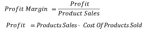
In the next example, let's assume you an Analyst at Adventureworks, you get a request call to provide the Profit Margin of products sold by Resellers. You pretend you know what is being asked of you, and then you google Profit Margin to come up with the formulas below.
The logic Listing 11 below shows how you translate the algorithm with DAX Queries by breaking it down into simpler calculations using Query Measures.
Listing 11:
DEFINE
    MEASURE 'FactResellerSales'[ProductSales] =
        SUM ('FactResellerSales'[SalesAmount])
    MEASURE 'FactResellerSales'[CostOfProductSold] =
        SUM ('FactResellerSales'[TotalProductCost])
    MEASURE 'FactResellerSales'[Profit] = [ProductSales] - [CostOfProductSold]
    MEASURE 'FactResellerSales'[ProfitMargin] =
        DIVIDE ( [Profit], [ProductSales] )
EVALUATE
SUMMARIZECOLUMNS (
    'DimProduct'[EnglishProductName],
    'FactResellerSales',
    "Profit Margin", 'FactResellerSales'[ProfitMargin]
)
As you can see from Listing 11, two Query Measures ProductSales and CostOfProductSold defined and hosted on the FactResellerSales are then subsequently used in the Profit calculations. The ProfitMargin measure simply invokes and divide the Profit and ProductSales measures. Finally, using the EVALUATE function, the product names are projected with ProfitMargin measure.
In the final example, we are going to learn a trick that lets you create arbitrarily shaped filters to use in your queries. Let's say you are often asked to filter the query in Listing 11 above. E.g. you are often asked to provide ProfitMargin for specific scenarios, like particular Resellers in a particular geography for particular years, etc. Normally one will have to use filter functions to achieve these results (similar to how we translated the SQL WHERE Clause above). In DAX there is a function, called TREATAS, that provides a way to add arbitrarily shaped filters to your query making such requests easy to reproduce.
In the example in Listing 12 below, the previous query in Listing 11 has been modified to add an arbitrarily shaped filter using the TREATAS function.
Listing 12:
DEFINE
    MEASURE 'FactResellerSales'[ProductsSales] =
        SUM ('FactResellerSales'[SalesAmount])
    MEASURE 'FactResellerSales'[CostOfProductsSold] =
        SUM ('FactResellerSales'[TotalProductCost])
    MEASURE 'FactResellerSales'[Profit] = [ProductsSales] - [CostOfProductsSold]
    MEASURE 'FactResellerSales'[ProfitMargin] =
        DIVIDE ( [Profit], [ProductsSales] )
EVALUATE
SUMMARIZECOLUMNS (
    'DimDate'[CalendarYear],
    'DimProduct'[EnglishProductName],
    'FactResellerSales',
    // Arbitrary filter
    TREATAS (
			 { ( 2013, "Progressive Sports" )
			  ,( 2012, "Progressive Sports" )
			 },
        'DimDate'[CalendarYear],
        DimReseller[ResellerName]
    ),
    // End Arbitrary filter
    "Profit Margin", 'FactResellerSales'[ProfitMargin]
)
In Listing 12 the query filters ProfitMargin for products specific to a Reseller named "Progressive Sports" for the years 2012 and 2013. The various filter parameters are passed to the query in Listing 11 by forming arbitrarily shaped filters with the function as shown below.
         // Start Arbitrary filter
        TREATAS (
                     {
                         ( 2013, "Progressive Sports" ),
                         ( 2012, "Progressive Sports" )
                      },
                     'DimDate'[CalendarYear], DimReseller[ResellerName]
         ),
        // End Arbitrary filter
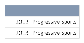
Note that the approach uses the DAX Table Constructor that allows you to define an anonymous table directly in code. The parenthesis { } represents the virtual table in this case two columns and two rows as below.
When applied in the query it creates a virtual relationship between a virtual table defined with specific virtual values to the base table (the expanded version). The result of the virtual table expression is passed as filters to columns passed as arguments in the TREATAS function, in this case, CalendarYear and ResellerName. Remember that these columns are columns in the extended version of the FactResellerSales base table ( please refer to the Expanded Table section in Part I ).
As we can see the TREATAS function offer one of the best ways to implement a virtual relationship in DAX queries. This approach is very useful if you have a small number of unique values to propagate in the filter. You can read more on DAX Table Constructor here and on the TREATAS function here.
Intro: DEFINE keyword
DEFINE introduces a query definition section that allows one to define local entities like tables, columns, query variables, and query measures that are valid for all the following EVALUATE statements. There can be a single definition section for the entire query, even though the query can contain multiple EVALUATE statements.
Query Variables
- Variables can be any data type, including entire tables.
- Query Variables cannot be used in Query Measures.
Query Measures
- In the definition of the measure, you must specify the table that hosts the measure.
- Query measures are useful for two purposes:
- To write complex expressions that can be called multiple times inside the query.
- They are useful for debugging and for performance tuning measures for instance before they are used in Power BI reports
Summary
After learning some fundamentals about DAX and the Tabular Model in Part I, we had set out to continue the learning process by understanding the functional nature DAX by simply translating SQL queries to DAX queries. We have accomplished that by translating all the causes in the SQL logical processing steps into DAX functional syntaxes.
Take-away
We learned that EVALUATE is the only required function to run a DAX query. Finally, we learned how to use the optional DEFINE parameter to define query variables and query measures that could be used as arguments or parameters within the body of an EVALUATE statement.
Essentially we were able to accomplish all DAX queries with three functions namely EVALUATE, SUMMARIZECOLUMNS and, FILTER. By learning how these three functions arguments to the summarized functional syntax below one can accomplish most of the DAX queries we wrote in this section.
EVALUATE( SUMMARIZECOLUMNS( FILTER() ))
Next
In the next installment of the series, we are going to take what we've learned from DAX queries into writing DAX calculations in the form of formulas that we will use in Power BI reports.